Data Grains Explained

This article is a discussion about source and output data granularity in Ready Signal. It goes over what data grains are and how they work.

• There two types of grains that determine at what granularity data is outputted in the system:
  • Time Grain: Day, Week, Month, Quarter Year
  • Geographic Grain: Zip, City, County, State, Country
• Source grain vs transformed output grain.
  • Source Grain is the granularity that the source data was created in.
  • Output grain is the grain you want your Signal output in.
  • The output grain is often not the same as the source grain.  
  • You have a few transformation options when moving from Source to Output grain:
    • Keep Data Source Granularity (Default)
    • Or Divide Evenly Based on Time (Time Grain) / Distribute Based on Population (Geo Grain)
  • Your Desired Output Grain is set at the Signal Level
    • This impacts the # of rows in your output and applies to all features
    • You can set the desired Time & Geo grains  when creating or editing a Signal
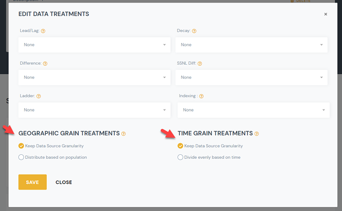
  • The Output Transformation settings are set at a Feature Level
    • You can have one feature where you Keep Data Source Granularity and another where you distribute based on population.
    • You can edit this value from the Manage Signal Details Page > Edit Treatments  Link
  • Read below for more detail on how these “Grain transformation” options work. 

• For Time Grain Treatments:
  • Keep Data Source Granularity (Default):
    • When the time source grain is different that the Time output grain, we repeat the same value by default.
      • Examples
        • Source grain is “monthly”, wtih a value of 10K, but the desired output grain is daily. We would show 10K for each day.
        • Source gain is “yearly”, value 8%, but output is weekly, we would show 8% for each week.
  • “Divide evenly based on time” (Optional):
    • This treatment allows you to spread a value evenly over a period of time. RS will do the simple algebra to spread it evenly.
    • If the value is a % you cannot divide it evenly, so even if you select divide evenly we will duplicate the number.
      • Example:
        • Unemployment rate of 9%,  has a monthly source grain. We will show as 9% at a daily grain regardless of time grain treatment.
      • If a value is a whole number, a total, then it can be divided evenly based over time.
        • Example:
          • New Home Sales where 30K in March.
          • Output = Daily Grain: Value for each day would be 1K (30K/30Days)
          • Output = Weekly Grain: Value for each week would be 7K

• For Geo Grain Treatments:
  • Keep Data Source Granularity:
    • When Source Granularity is LARGER than the Output granularity:
      • We repeat the same value.
      • Examples
        • Source grain is “state”, value w 10K, but output is city. We would show 10K for each city.
        • Source grain is “country”, value is 9%, but output is state. We would show 9% for each state.
      • When Source Granularity is SMALLER than the Output granularity:
        • If it’s a whole number, we do sum to the output granularity
          • Example:  Source grain zip but output is state.  We sum to state.
        • If it’s a Percentage, we take the weighted average
          • Example: Source grain zip but output is state.  We take the weighted average to state [sum((percentage * population))/sum(population)].
  • “Divide evenly based on population” (Optional)
    • This treatment allows you to spread a value over different geographies based on population levels.
    • If the value is a % you cannot spread it out, so even if you select divide evenly based on population we will duplicate the number.
      • Example:
        • Unemployment rate of 9%,  has a state source grain. We will show as 9% at a zip code level for all zips in that state.
      • If a value is a whole number, a total, then it can be divided proportionately based on population.
        • Example:
          • If that input is at the state level and the output is at the zip level.  [State level value]*(Zip Population /State Population)
• Additional topics:
  • Census data comes in at track level, we turn it to Zip then, sum up
  • Weather data, comes in by weather stations. We assign a weather station to each zip based on proximity.
  • Weather data can be rolled up based on population (how people experience the weather) or square miles (how the land experiences weather).